Optional: Count-Min Sketch

Tip

This slide is optional! It’s a cool application of hashing to solve a problem that works with large datasets, but the specifics are a little outside the scope of our course.

---

While hashing is most commonly used in applications such as making set and dict have constant-time lookup, hashing has an incredible number of applications to helping algorithms scale to large datasets. To see one such example of using hashing in a large-data application, we will focus on the task of counting.

At our startup Schmoogle, we provide a search engine for the world to use. While we ostensibly care about user’s privacy at our company, we care more about making money. To that end, we want to ensure we are able to record the most frequently searched queries so we can better monetize popular searches.

A very simple approach is to use a dict to use keys for queries and values for counts. Each time a new query comes in, we can just increment the count for that key by one (or storing 1 if its the first time using this query). How many key/value pairs will this dict have? The number of unique queries in the system (e.g., 'dogs' , 'adorable dogs' , 'very cute dogs' , etc.).

At Schmoogle, this is probably fine since we only have one user (my mom is very supportive of my business endeavors, I guess). Would this approach work for Google, our biggest competitor? This will surely be very difficult to manage since the sheer volume of searches they receive. In 2017, Google received over 2 trillion searches, 15% of which were never-seen-before ( source )! That is a lot of keys! You can imagine they would quickly run out of memory on a single computer to store this dict .

So a clever idea is to try to save space by only trying to approximate the count. Instead of asking that our count is exactly the number of times a query has appeared, we only ask that the count is close to the true count. We can accomplish this by using a hash table that doesn’t use separate chaining, and instead just stores a count at each index like in the picture below.

Say a new query for 'dog' comes in. We start by hashing it to it’s proper index using its hash function. Say that ends up going to index 4. We would then go to that index and increment that count by one to indicate a new query has come in (\(77 \rightarrow 78\)).

So now if we want to find approximately how many times a query has been searched, we can just look up its index in the hash table. Say we want to find the approximate count for the query 'cat' (index 6). We look it up and see value 17. Now,17 is not the true count of 'cat' since it’s likely another query collides at that index. Our hope though, is that this count is not too far away from the truth. This count has the property that it’s always an over-estimate of the true count since an error only occurs if another query collides with that one.

This idea of using a data structure to approximate information about a dataset is called sketching . With a sketch, we get a loose idea about the data without needing to have all the particular details. With a sketch, these counts will be approximations of the true counts. As we mentioned before, errors will only come from collisions so one way to reduce the errors could be to use a better hash function and a larger hash table. An incredibly clever idea that works well in practice takes an entirely different approach: use multiple hash tables!

Count-Min Sketch

The idea is to use \(d\) different hash tables with \(w\) slots in each as shown in the image below. Each hash table will use a different hash function. Every time we receive a new query, we increment the count in its correct place in each hash table.

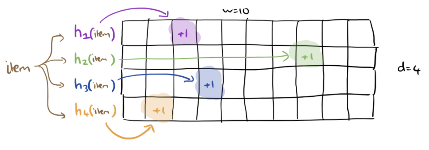
When we want to look up the count for an item, we look up its counts in each of the hash tables.

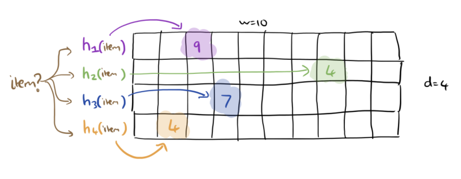
In the image above, we see a count of 9, 4, 7, and 4. What should we say the count of the given item is? Well, since each hash table is an over-estimates of the count based on its set of collisions for that index, we know that the four counts we see are all over-estimates. In that case, our best guess is to report the smallest number we see out of these four counts. In this case, we will report the count of the item is 4.

This algorithm is called count-min sketch since it takes the minimum of multiple count sketches. The reason this actually works comes from the fact that each hash table uses a different hash function. The trick for why using multiple hash tables with different hash functions will help us is that it is unlikely for the same items to collide in the exact same ways in different hash tables. So even if 'dog' and 'cat' collide in one table, it’s unlikely they will collide with each other in other tables! With some math you can quantify how large you expect the errors to be.

This approach works great if you can tolerate errors. For example, if your website wants to display the number of times a particular page was viewed, it’s probably tolerable if that count is off by a small amount. If instead, you were trying to keep track of payments made, this would be a terrible thing to use since that is not a context where an error is tolerable.

The savings of memory can be huge though which might be something you prioritize. Using the plain dict approach, you would require \(\mathcal{O}(n)\) memory usage where \(n\) is the number of queries. With this count-min sketch structure, you can approximately answer queries with only \(\mathcal{O}(wd)\) space. Your error decreases if you use a larger \(w\) or \(d\), but the space savings can still be quite great even with a larger structure. Just a sense of scale, you can take something that would require 32GB of memory with a dict down to just 32KB while only incurring small error.