Why Convolutions?
Contents
Why Convolutions?#
Consider trying to write a program to solve the task of determining if a given image contains a dog or a cat. This might sound familiar as it was the first problem we described as an example of a machine learning system! While that was our first example, it turns out that machine learning with images is pretty tough to do well. The reason stems from the fact that it’s not obvious which features you should use for the model since you are given just a bunch of pixels. We will talk more about how to do ML with images in the next lesson, but we wanted to take some time now to motivate why learning convolutions is important.
In the past, one of the things computer vision experts used to do to solve this task was try to make features from convolutions of different kernels (e.g., is there a corner here, or is there an edge here). Once they hand-specified a set of kernels to use on an image, they would run convolutions on them to get their features and then use some machine learning algorithms to learn from those features. The intent behind this approach is that these kernels they specified (e.g., edge detector) formed some set of meaningful, low-level features. This worked okay, but we quickly hit a road-block with the performance of these models that used these hand-specified features.
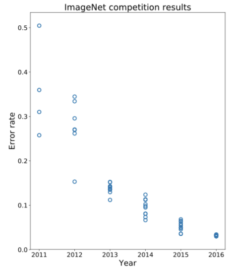
A common competition to test computer vision systems, ImageNet, recorded the error in classifications for various models in its competition each year it was hosted. The competition has images from thousands of labels, and the models are tested on their ability to correctly predict those labels from the image alone. Before 2012, the state of the art systems were hovering around 30% error on the ImageNet challenge. An example of a “breakthrough” in the field at that time would be to improve the error by 1% or so. Then, in 2012 we saw a drastic decrease in the error on ImageNet with one submission getting about ~15% error. The graph below shows this jump in error in 2012 and a steady decrease in the error over time.
The breakthrough in 2012 was the introduction of a system that uses deep learning (this buzzword you may have heard in the news). We will talk a bit more about what these deep learning models try to do in the next lesson. The more important point for us is that this model used a design called a convolutional neural network to drastically improve its accuracy. The idea behind this model is to have a series of convolutions performed on the data, but kernels that are learned by the model itself! Instead of having an expert hand-specify that some kernel computes edges, the model would learn its own set of kernels that worked best for the task at hand! This idea was so successful in image classification tasks, that almost every state-of-the-art system for image recognition today uses this type of model!
Has it all been solved?#
Looking at the graph above, we can see in 2016 we are hitting near human-level performance in these systems. Since they are performing so well, you might be wondering if classifying images is a solved problem since it’s not obvious that these models should be able to do better than humans at a task like visual perception. Since they do so well on this challenge, we would hopefully expect they will do well in other perception tasks, like the ones required for self-driving cars.
Unfortunately, we are quite a ways away from being done! It turns out that while these models do very well in this constrained problem of ImageNet, they start behaving very poorly if you go slightly out of that domain. A pretty shocking example is shown in the image below. If you take an image of a panda, a model that does well on ImageNet can predict it’s a panda with some confidence (since “panda” was one of the labels in the data it learned from). Now, imagine adding a bit of noise to the image in the sense that you change the pixel values by a very small amount so that the image still visually looks the same to humans. Now, if you take this modified image and ask the model to predict it, we have seen that it will very confidently say that the picture is of something else, like a gibbon!
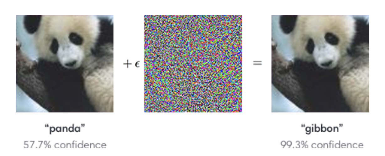
Not only did the model make a mistake on this example, but it also very confidently made a mistake! This should cause us some pause when thinking about using these models in self-driving cars. What if the lighting in the world suddenly changes because it gets cloudy, and now our model now confidently thinks stop signs are green lights!
This fear is also embodied by one of my favorite tweets. In reality, the reason you click on images of stop signs in captchas is to provide more labeled training data of images; they give you images taken at weird angles or different lighting to help make the models more robust. Nonetheless, it’s still terrifying that slight changes can cause wildly different outputs!