Revisiting Time Efficiency

---

Last time we introduced the notion of efficiency, namely in terms of time taken to run the program. We saw that time was unreliable and that computer scientists instead discuss an algorithm’s efficiency in terms of its Big-O notation. Today, we will discuss some limitations of Big-O notation and highlight the importance of why it is used (since it is often misunderstood).

For example, consider the following code snippet that shows three different methods for computing the maximum difference between any pair of values in a list.

def max_diff1(nums):
    # Find the max difference between any pair of nunber
    max_diff = 0
    for n1 in nums:
        for n2 in nums:
            diff = abs(n1 - n2)
            if diff > max_diff:
                max_diff = diff
    return max_diff

def max_diff2(nums):
    # Realize the max difference is the same as the max
    # number minus the min number
    min_num = nums[0]
    max_num = nums[0]
    for num in nums:
        if num < min_num:
            min_num = num
        elif num > max_num:
            max_num = num
    return max_num - min_num

def max_diff3(nums):
    # Same as max_diff2 but uses Python built-ins
    return max(nums) - min(nums)

What are the Big-O run-times of each of these functions? Let \(n\) be the length of the input list.

• For max_diff1 , the runtime is \(\mathcal{O}(n^2)\).

• For max_diff2 , the runtime is \(\mathcal{O}(n)\).

• For max_diff3 , the runtime is \(\mathcal{O}(n)\).

So according to Big-O, max_diff1 is clearly the worst while max_diff2 and max_diff3 are equivalent. We’ll see that this might not be all to this story.

You have to be a bit careful when considering Big-O notation since it has some specific uses and some specific drawbacks.

• Pros

  • It clearly describes how an algorithm will scale (e.g., if you double the input, it will take X time longer).

  • The Big-O notation is independent of the programming language you are writing in or the computer you are writing the program on. When considering raw time taken by a program to run, these factors have a huge impact on the run-time of the program.

  • Easy to figure out by just looking at the code (with practice 😊).

• Cons

  • It can be overly-simplistic. It’s not actually the case that every step takes the same amount of time (e.g., multiplication is actually slower than addition).

  • The coefficients and lower-order terms we drop can sometimes have a BIG impact on performance.

To understand the last point, consider the algorithm for matrix multiplication that you might use in a linear algebra class. Don’t worry, you don’t need to understand what matrix multiplication is, but just know it’s a problem that there is an algorithm to tell you the answer for multiplying two \(n \times n\) matrices. The algorithm that you would learn in a linear algebra class is sometimes called the “naive” algorithm, which takes \(\mathcal{O}(n^3)\) time.

This operation is so important in computing in science, \(\mathcal{O}(n^3)\) does not suffice for many modern applications where \(n\) is large. Many researchers have spent their careers trying to find asymptotically faster algorithms. In the graph below, we show the progress on finding algorithms that scale faster than \(\mathcal{O}(n^3)\). The x-axis shows years and the y-axis shows \(\omega\) which represents the exponent in \(\mathcal{O}(n^\omega)\).

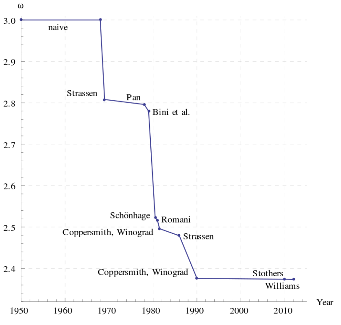
Although recent advancements in algorithm design have found algorithms to do matrix multiplication in time less than \(\mathcal{O}(n^{2.5})\), those algorithms are rarely used in practice! The reason is that the coefficients that \(\mathcal{O}(n^{2.5})\) hides are so large, that the run-time still ends up being way slower than a simpler algorithm with a larger exponent. So while these algorithms are asymptotically faster (as \(n\) goes to infinity), in practice for sizes of \(n\) that can actually fit on a computer, sometimes an asymptotically slower algorithm is faster because there are lower coefficients.

For a concrete example, consider how \(2n^2 \leq100n\) for all \(0 \leq n \leq 50\). So while the \(\mathcal{O}(n)\) equation on the right-hand side is asymptotically faster than the \(\mathcal{O}(n^2)\) on the left, the coefficient it hides can make it slower for some smaller \(n\).

In the next slide, we will see another tool that can help us understand the performance of our programs.