Practice: Time Series

Jupyter Info

Reminder, that on this site the Jupyter Notebooks are read-only and you can’t interact with them. Click the button above to launch an interactive version of this notebook.

• With Binder, you get a temporary Jupyter Notebook website that opens with this notebook. Any code you write will be lost when you close the tab. Make sure to download the notebook so you can save it for later!

• With Colab, it will open Google Colaboratory. You can save the notebook there to your Google Drive. If you don’t save to your Drive, any code you write will be lost when you close the tab. You can find the data files for this notebook below:

  • google.csv

You will need to run all the cells of the notebook to see the output. You can do this with hitting Shift-Enter on each cell or clicking the “Run All” button above.

In this notebook, we use a few features of this library called matplotlib (renamed as plt) to save a plot to a file. You do not need to understand this part and can leave those parts of the code untouched. We will discuss matplotlib in the next module!

Fig. 1 How I assume the stock market works

In this problem we will be working with stock-market data. Don’t worry, you don’t need to understand how stocks work to do this problem (Hunter sure doesn’t!). All the background you need to know is that a higher number corresponds to more value (money), and a lower number corresponds to less value (money).

import pandas as pd
import matplotlib.pyplot as plt

# A special magic command to make plots work in the notebook
%matplotlib inline

Problem 0

Load in the Google stocks dataset from the file google.csv so that the Date column becomes the time-series index.

For testing purposes, store the result in a variable called goog.

You might also want to make sure you display goog.head() so you can get an idea what the DataFrame looks like.

# Write your code here!

For this notebook, we will only be looking at the column Adj Close that represents the value of the stock at the end of the day. Whenever we ask you to plot something, you should grab the Series for that column and plot with the plot function in it (e.g., df['col'].plot())

Problem 1

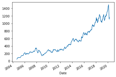
Use the plot function to plot the Adj Close column for the entire dataset.

Do not customize your plot in any way for this problem, since we will compare it to the plain plot.

Your plot should look like the plot below:

# Write your code below this comment and above the next comment!


# Write your code above this line!
plt.savefig('/home/prob1.png')

Problem 2

Let’s get a closer look to see how the Covid-19 pandemic impacted Google’s stock price. Select the subset of the data from October 2019 (month 10) to April 2020 (month 4). You should not specify any days in your indexing. Store your result of the Adj Close prices for this range of dates as a Series.

For testing purproses, store your result in a variable called ans2.

At the end of the testing cell, we plot your ans2 to visually inspect the change in the stock price.

# Write your code below this comment and above the next comment!


# Write your code above!
ans2.plot()

Problem 3

To remove some of the noise, let’s change the frequency of the data from daily to monthly to see how Google has done year to year.

Compute the monthly average value for the column Adj Close. Your result should be a Series indexed by each month over the 15 or so years of data and each value is the average value for all rows that belonged to that year.

For testing purposes, store the result in a variable called ans3.

Your plot will look somewhat similar to the plot in plot 4 (but will be a little smoother).

Hint: Look at the reading before to see how we change the time-frequency of a time-series dataset.

# Write your code below this comment and above the next comment!



# Write your solution above!
ans3.plot()

Problem 4

For this problem, we are going to be a little adventurous and have you explore some documentation to learn how to use a new pandas function. We highly recommend that you start by reading the brief description at the top and then looking down at the examples. There is NO way that you will read this and understand every parameter available or all the syntax they use, but you WILL be able to look at an example and translate it to what you need.

For this problem, we want to compute a rolling average of the data over a two-week period. Recall that each row corresponds to a single day so two weeks corresponds to 14 days. This is different than a resample operation since for each day, it will take the average of the last 14 days (hence why it’s called a rolling average).

Your result should be a Series with the same index. The first few rows should be NaN as the documentation linked in the last paragraph suggests in their examples (since there is not enough data for the rolling average at the start).

For testing purposes, store the result in a variable called ans4.

Your result should look something like the following and when plotted should look like the plot below (check the output after your code cell).

Date
2004-08-19            NaN
2004-08-20            NaN
2004-08-23            NaN
2004-08-24            NaN
2004-08-25            NaN
                 ...     
2020-04-07    1125.788565
2020-04-08    1132.573565
2020-04-09    1142.511422
2020-04-13    1154.007141
2020-04-14    1163.633571
Name: Adj Close, Length: 3940, dtype: float64

# Write your code below this comment and above the next comment!



# Write your solution above
ans4.plot()
ans4