Time Series
Contents
Time Series#
Jupyter Info
Reminder, that on this site the Jupyter Notebooks are read-only and you can’t interact with them. Click the button above to launch an interactive version of this notebook.
With Binder, you get a temporary Jupyter Notebook website that opens with this notebook. Any code you write will be lost when you close the tab. Make sure to download the notebook so you can save it for later!
With Colab, it will open Google Colaboratory. You can save the notebook there to your Google Drive. If you don’t save to your Drive, any code you write will be lost when you close the tab. You can find the data files for this notebook below:
You will need to run all the cells of the notebook to see the output. You can do this with hitting Shift-Enter on each cell or clicking the “Run All” button above.
We start by loading the biycycles dataset into a DataFrame using the same code as in the last slide to index the data by the date.
# Some setup code to get the plotting library correct
import matplotlib.pyplot as plt
import pandas as pd

%matplotlib inline
df = pd.read_csv('bicycles.csv',
                 index_col='Date', parse_dates=True)

# Sorts the rows so the index is sorted
df = df.sort_index()

df  # For display
| East | West | |
|---|---|---|
| Date | ||
| 2012-10-03 00:00:00 | 4.0 | 9.0 |
| 2012-10-03 01:00:00 | 4.0 | 6.0 |
| 2012-10-03 02:00:00 | 1.0 | 1.0 |
| 2012-10-03 03:00:00 | 2.0 | 3.0 |
| 2012-10-03 04:00:00 | 6.0 | 1.0 |
| ... | ... | ... |
| 2019-03-31 19:00:00 | 30.0 | 58.0 |
| 2019-03-31 20:00:00 | 26.0 | 31.0 |
| 2019-03-31 21:00:00 | 18.0 | 15.0 |
| 2019-03-31 22:00:00 | 7.0 | 14.0 |
| 2019-03-31 23:00:00 | 6.0 | 10.0 |
56904 rows × 2 columns
Just like with any other pandas object, we can inspect the index of this DataFrame using the .index attribute.
df.index
DatetimeIndex(['2012-10-03 00:00:00', '2012-10-03 01:00:00',
               '2012-10-03 02:00:00', '2012-10-03 03:00:00',
               '2012-10-03 04:00:00', '2012-10-03 05:00:00',
               '2012-10-03 06:00:00', '2012-10-03 07:00:00',
               '2012-10-03 08:00:00', '2012-10-03 09:00:00',
               ...
               '2019-03-31 14:00:00', '2019-03-31 15:00:00',
               '2019-03-31 16:00:00', '2019-03-31 17:00:00',
               '2019-03-31 18:00:00', '2019-03-31 19:00:00',
               '2019-03-31 20:00:00', '2019-03-31 21:00:00',
               '2019-03-31 22:00:00', '2019-03-31 23:00:00'],
              dtype='datetime64[ns]', name='Date', length=56904, freq=None)
So now to get a row for a particular date and time, we can index into the DataFrame using loc! The key difference here is that we will specify a string for the date-time rather than a number (since the index is the date-time).
df.loc['2019-03-31 15:00:00']
East    130.0
West    121.0
Name: 2019-03-31 15:00:00, dtype: float64
The incredibly powerful thing about using date-time as the index type is it allows us to do semantic indexing based on dates and times. Here are some examples:
You can pick just a date and it will include all rows from that date (meaning it will have all the times for that day).
df.loc['2017-03-31']
| East | West | |
|---|---|---|
| Date | ||
| 2017-03-31 00:00:00 | 2.0 | 4.0 |
| 2017-03-31 01:00:00 | 2.0 | 0.0 |
| 2017-03-31 02:00:00 | 1.0 | 0.0 |
| 2017-03-31 03:00:00 | 1.0 | 0.0 |
| 2017-03-31 04:00:00 | 3.0 | 3.0 |
| 2017-03-31 05:00:00 | 23.0 | 14.0 |
| 2017-03-31 06:00:00 | 57.0 | 49.0 |
| 2017-03-31 07:00:00 | 163.0 | 99.0 |
| 2017-03-31 08:00:00 | 250.0 | 162.0 |
| 2017-03-31 09:00:00 | 90.0 | 70.0 |
| 2017-03-31 10:00:00 | 52.0 | 38.0 |
| 2017-03-31 11:00:00 | 39.0 | 31.0 |
| 2017-03-31 12:00:00 | 37.0 | 37.0 |
| 2017-03-31 13:00:00 | 52.0 | 34.0 |
| 2017-03-31 14:00:00 | 45.0 | 55.0 |
| 2017-03-31 15:00:00 | 74.0 | 87.0 |
| 2017-03-31 16:00:00 | 83.0 | 223.0 |
| 2017-03-31 17:00:00 | 145.0 | 333.0 |
| 2017-03-31 18:00:00 | 117.0 | 206.0 |
| 2017-03-31 19:00:00 | 50.0 | 84.0 |
| 2017-03-31 20:00:00 | 26.0 | 36.0 |
| 2017-03-31 21:00:00 | 16.0 | 40.0 |
| 2017-03-31 22:00:00 | 12.0 | 22.0 |
| 2017-03-31 23:00:00 | 5.0 | 15.0 |
You could also leave off the day to get all of the rows for a year and month.
df.loc['2017-03']
| East | West | |
|---|---|---|
| Date | ||
| 2017-03-01 00:00:00 | 1.0 | 2.0 |
| 2017-03-01 01:00:00 | 2.0 | 2.0 |
| 2017-03-01 02:00:00 | 1.0 | 1.0 |
| 2017-03-01 03:00:00 | 1.0 | 0.0 |
| 2017-03-01 04:00:00 | 3.0 | 3.0 |
| ... | ... | ... |
| 2017-03-31 19:00:00 | 50.0 | 84.0 |
| 2017-03-31 20:00:00 | 26.0 | 36.0 |
| 2017-03-31 21:00:00 | 16.0 | 40.0 |
| 2017-03-31 22:00:00 | 12.0 | 22.0 |
| 2017-03-31 23:00:00 | 5.0 | 15.0 |
744 rows × 2 columns
Unsurprisingly, you can also just get all the rows for a year. All of these examples are accomplished by interpreting the value you are using to index as a date-time, and then selecting all the rows that match that date-time. If you just specify a year, it finds all rows that have that year.
df.loc['2017']
| East | West | |
|---|---|---|
| Date | ||
| 2017-01-01 00:00:00 | 0.0 | 5.0 |
| 2017-01-01 01:00:00 | 5.0 | 14.0 |
| 2017-01-01 02:00:00 | 1.0 | 0.0 |
| 2017-01-01 03:00:00 | 0.0 | 2.0 |
| 2017-01-01 04:00:00 | 0.0 | 1.0 |
| ... | ... | ... |
| 2017-12-31 19:00:00 | 9.0 | 12.0 |
| 2017-12-31 20:00:00 | 6.0 | 8.0 |
| 2017-12-31 21:00:00 | 3.0 | 10.0 |
| 2017-12-31 22:00:00 | 7.0 | 6.0 |
| 2017-12-31 23:00:00 | 7.0 | 9.0 |
8760 rows × 2 columns
You can also use ranges to select multiple years!
df.loc['2017':'2018'] # All rows from 2017 to 2018 (inclusive for pandas)
| East | West | |
|---|---|---|
| Date | ||
| 2017-01-01 00:00:00 | 0.0 | 5.0 |
| 2017-01-01 01:00:00 | 5.0 | 14.0 |
| 2017-01-01 02:00:00 | 1.0 | 0.0 |
| 2017-01-01 03:00:00 | 0.0 | 2.0 |
| 2017-01-01 04:00:00 | 0.0 | 1.0 |
| ... | ... | ... |
| 2018-12-31 19:00:00 | 9.0 | 5.0 |
| 2018-12-31 20:00:00 | 12.0 | 14.0 |
| 2018-12-31 21:00:00 | 7.0 | 7.0 |
| 2018-12-31 22:00:00 | 3.0 | 4.0 |
| 2018-12-31 23:00:00 | 7.0 | 6.0 |
17520 rows × 2 columns
Plotting#
In Lesson 10, we will spend time discussing how to plot data and how to interpret those visualizations. pandas provides some basic functionality for plotting.
df.plot()
<matplotlib.axes._subplots.AxesSubplot at 0x7f3d35ecdc40>
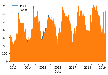
This is not exactly readable… The problem is the data is too “high resolution”: it’s drawing a line for every hour of every day for 6 years! No wonder we can’t actually see anything.
What we need is to “resample” the data so the data points occurr less frequently. One way to do this would be to just drop every row besides Sundays at 12pm (arbitrarily decided), but you can tell that won’t work because it won’t give us a good idea of overall biking trends. Instead, it would be nice if we could re-organize the data so each row was the total number of bikers in a week (just for example).
This sounds somewhat similar to a group-by, but turns out to work quite differently (more on this in next section). To change the time series to have the granularity of every week and then plot that, we use the resample method. In the next cell, we transform the data so each row is a time-span of a week and has the sum of all the bikers for the hours in that week.
weekly = df.resample('W').sum()
weekly.plot()
<matplotlib.axes._subplots.AxesSubplot at 0x7f3d354c6280>
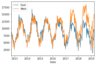
Much more legible! Now we can see both East and West traffic. Looking at the graphs, we see some seasonality in the data - there are peaks in the summer and troughs in the winter.
'W' is a special code for resample to tell it to resample by week. There are many other codes you can pass to it instead!
'D'= day'W'= week'M'= month'A'= year
Generally when analyzing time series, you are interested in looking at two metrics of describing the series.
Its trend, which shows how the average value changes over time. This dataset seems to have no obvious upward or downward trend (the average number of bicyclers, in say a year, are about the same).
Its seasonality, which shows how the sequence fluctuates over some period. This series definitely has some seasonality to it since it goes up and down in relatively the same pattern each year.
Resample vs Group By#
Earlier, we showed that to change the time series to be by week, instead of by hour, we used a resample. We commented that we didn’t actually want to use groupby because these are fundamentally different operations.
To show you that these in-fact, are different, we can try using a groupby to solve the problem. If we want to access the week for each row, we can use df.index.week. df.index returns the date-time index and .week gets the week value from each row. The week value will be a number from 0 to 52, indicating which week that date-time is in.
In the cell below, we groupby this week value and then plot the result.
weekly_groupby = df.groupby(df.index.week).sum()
weekly_groupby.plot()
<matplotlib.axes._subplots.AxesSubplot at 0x7f3d354a3c70>
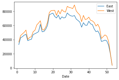
Wow! Why does that look so different?!?!
It has to do with how groupby works and the fact that we tried to group by the week-number. As we said before, df.index.week will be a Series of numbers between 0 and 52, indicating which week the date-time fell in. However, this causes a problem for the same week in different years!
Consider Jan 2, 2018 and Jan 5, 2019. Both of those .week values will be 0 since they are in the first week! The year information was lost! They will end up landing in the same group, which is why we can see that graph only goes from 0 to 52!
Instead, we want to do some kind of grouping based on the weeks themselves. We want Jan 2, 2018 and Jan 5, 2019 to go into separate groups with their respective date-times that are in the same week.
While it is actually possible to try to put something together that works and uses groupby, we will not go into that here. Instead, resample is an operation precisely meant to make this easier! You just tell pandas you want to resample by week, and it figures that out for you!
There is a lot more complexity you can get into with time series. For example, resample turns out to be much more complicated since you can use it to downsample (throw away data) or upsample (create new data) so that the data are sampled at the desired frequency. There are too many details to go into that here, but you may learn more from pandas documentation!