Convolutions
Contents
Convolutions#
So far we have seen some very simple ways of transforming images. In this slide, we will describe a very useful type of operation done in image analysis to help extract local information in an image. An example of local information would be something like “is there an edge in this part of the image?” This type of approach for analyzing images has been instrumental in building state-of-the-art image recognition systems used today (more on this later). The type of operation we are going to describe here is called a convolution.
The idea of a convolution follows from it being a sliding window algorithm: an algorithm that moves through the data looking at a certain-sized region of the data at a time. A convolution is a special type of sliding window algorithm that we run over an image. In a convolution, we use another 2D array, called a kernel, that we use to compute a value for each location. The result of a convolution is a smaller “image” that stores the result of the computation for each sub-region. This is much easier to understand visually with an example.
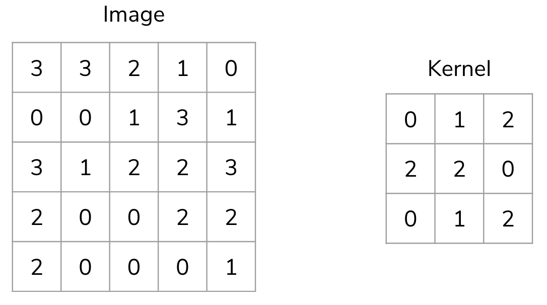
Suppose I had the following input image (a (5, 5) numpy.array ) and a smaller 2D array that we will use as the kernel (a (3, 3) numpy.array ).
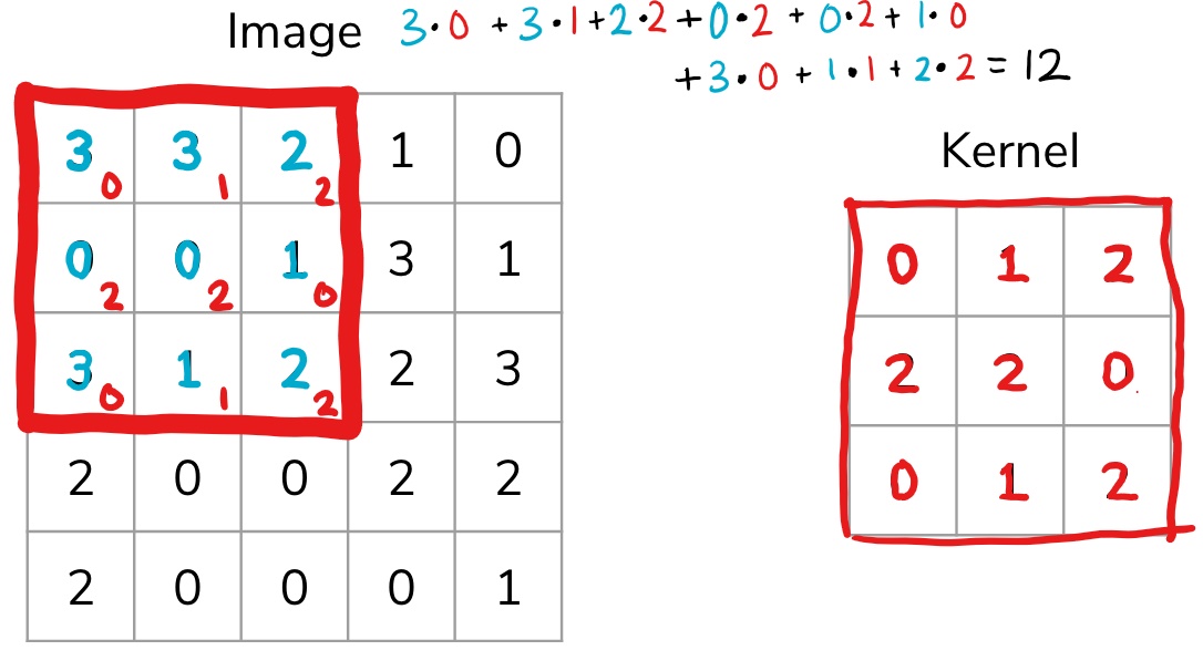
We start by overlapping the kernel at the top-left of the image shown in the image below. We compute an element-wise product between the kernel and the part of the image it overlaps with and then compute the sum of those values to be the result for this location. So the image below shows the sum of the element-wise product being 12 for that position of the kernel over the image. We then move the kernel to the right one position and repeat this process. Once, it reaches the right side, it goes back to the left but starts one row lower until it’s hit every possible part of the image.
This whole process is best seen in an animated fashion to show all locations the kernel visits. In the GIF below, the blue image is the original image, the darker blue area is where the kernel currently is (and its values are shown in the bottom right of each cell), and the resulting image is shown in green.
Notice how this convolution computes a value for each part of the image. This is what we mean by “local information”. The kernel (which you choose) computes some value for each part of the image, and the result can then be used to do some analysis based on those values.
You are probably thinking that these kernel numbers don’t make a lot of sense and this process doesn’t seem that useful, which is fair. However, you can do some pretty clever things using this approach depending on which kernel you use!
Types of Kernels#
There is a bit of an art to deciding how big (i.e. its shape) the kernel should be or what numbers you should use inside of it. For a while in the late ’90s and early ’00s, computer vision experts spent a lot of time hand picking numbers that seemed to work in practice with okay performance. Nowadays we use machine learning to learn the kernel values for us!
The image below has some example kernels that are used in practice and what they are used for. We won’t explain all of them because the numbers themselves aren’t important. The cool thing is that all of the operations they implement (edge detection, sharpen, box blur) are all different from our perspective, but are actually just the same convolution operation with different kernels!
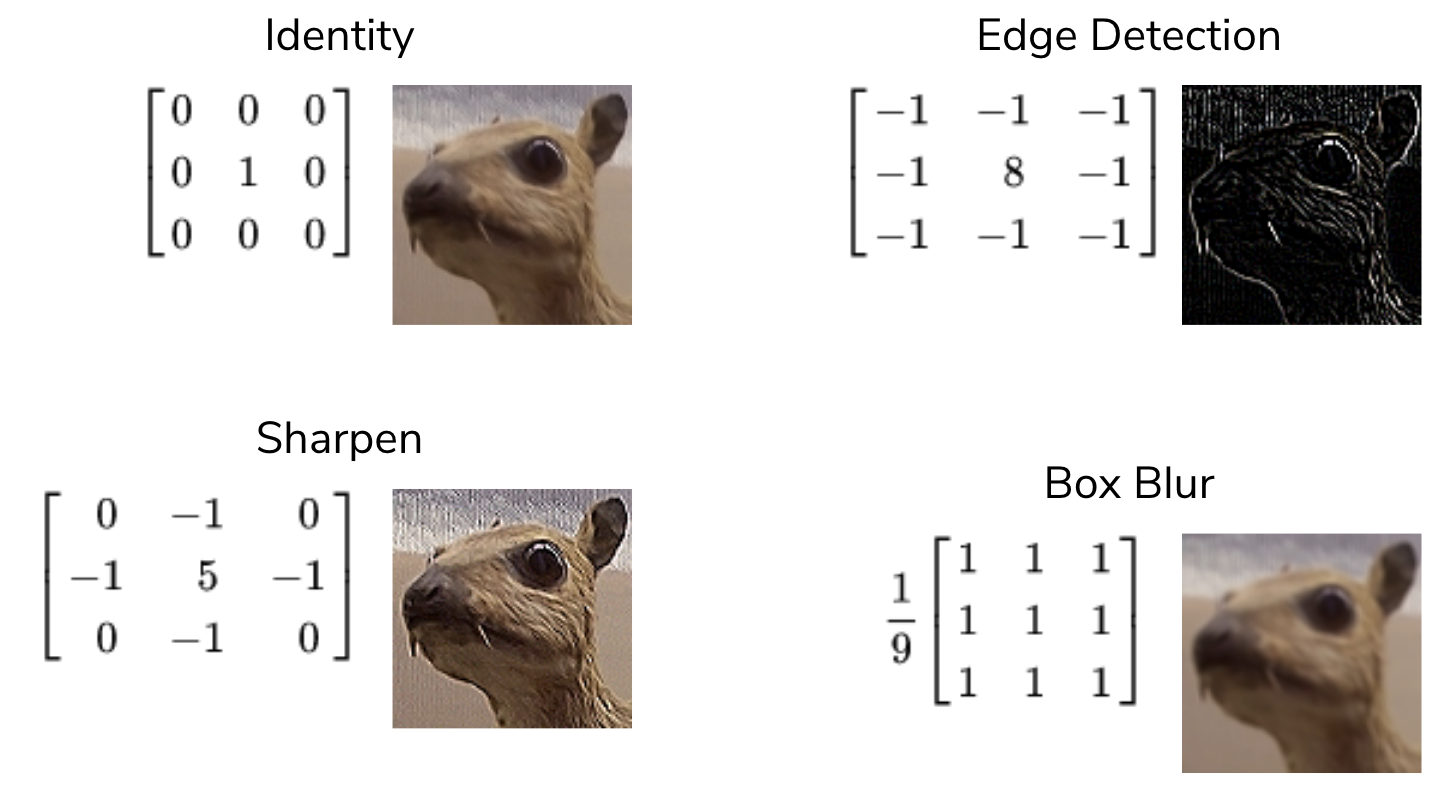
To get an intuition for why these do what they do, consider the edge detection kernel. It has the value 8 in the middle and -1s all around it. This kernel helps detect edges. What this means is that in the resulting image, places with high values (showing up as white in the image above) correspond to edges in the original picture.
Why does this kernel accomplish this? Consider an image that was all the same shade of blue for all pixels in the image. This image would clearly not have any edges in it since all pixels are the same color! If we think of a convolution using this kernel, at every location, the kernel overlaps with the image, the result will be 0! You can convince yourself of this since any pixel value in the center will add 8 of itself to the result, but then its 8 surrounding pixels would contribute -1 of themselves to the result. Conversely, the result using this kernel is non-zero when there is a large difference in the color at the center and those around it. This is exactly why this kernel detects edges!
Code Consideration#
The rules of Python being slow still apply to numpy: you want to avoid loops whenever possible. It turns out that for convolutions, there is not a clean way of writing this sliding window algorithm without loops. You’ll get practice writing code with loops in the practice problem for this lesson.
Your Task#
To reiterate, understanding the specific numbers in these kernels or why they compute what they do is not incredibly important. For us, the important part is the algorithm to compute the result of a convolution using some given kernel. The reason is we want you to be familiar with this algorithm since it has many different applications in image analysis (primarily in applications of machine learning to image analyses). This can be something helpful or interesting to look at in your project. So for this lesson, the goal will be to practice our understanding of convolutions and get some practice with numpy code with images!