Binary Search Tree

---

Let’s change examples for a second before going back to efficiently finding a user profile for Spacebook.

Pretend for a moment that we are nearing the end of November. Yesterday was Thanksgiving and Hunter decided to go Black Friday shopping to buy a new Supreme shirt. Say you get to the rack with the shirts and notice they are sorted by size like in the image below. Now our picture shows only 5 shirts, but imagine there are hundreds and hundreds of them (sorted by size), and we can’t tell the size without looking at the tag on the shirt.

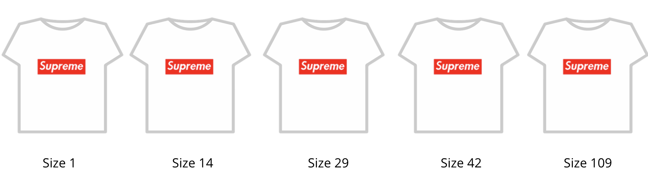
Now Hunter knows he is a size 42 and his goal is to make it out of Black Friday alive by finding the shirt in his size as quickly as possible before the crowd stampedes. If Hunter knows his shirt size is 42, would the optimal strategy be to start at the smallest shirt size (1) and go shirt by shirt until he finds his size? Not if he is trying to survive!

You probably have a good heuristic to help you find your shirt more quickly than that: start in the middle! If you look at the shirt in the middle of the rack, say size 29, you know that Hunter’s shirt size (42) will be after the mid-point since 42 is larger than 29. This enables you to eliminate half of the shirts to look at since there is no way that Hunter’s shirt is before the shirt of size 29, assuming the shirts are sorted by size. You can repeat this process again by picking the mid-point of the remaining shirts. This algorithm of repeatedly going to the mid-point and going left or right from that is called binary search. The algorithm, written in pseudo-code looks like the following:

Input: List of shirts sorted by size and a target value to find

while there are more than 1 shirt remaining:
    mid = the shirt size of the shirt in the middle
    if target == mid:
        buy the shirt!
    else if target > mid:
        throw out all the shirts of size < mid
    else: # target < mid
        throw out all the shirts of size > mid

If we made it outside this loop and still haven't found the shirt,
  we can report that the shirt size is not in the list of shirts

We call this algorithm binary search because it splits the group in half and eliminates half the choices each time (binary means having 2 possible choices).

We can use this exact strategy to find the Spacebook user from the user ID as long as we make sure the list of users is sorted by user ID! Now the question is: Is this binary search procedure more efficient?

Binary Search Efficiency

All of the steps inside the loop of our pseudo-code are constant time; there is no looping involved in the body so the run-time of this algorithm is going to depend on the number of times this while loop runs. Notice, on every iteration of the algorithm, we eliminate half of the choices and we stop once there are 1 or fewer items. This means our run-time is going to be related to the number of times the number of elements in the list \(n\) can be divided by 2. Mathematically, this can be written as finding the number of times we need to run \(n / 2 / 2 / ... / 2 = 1\).

It’s probably not obvious how to tell how many times we can divide a number by 2. It helps to use a bit of algebra to solve this. Call the number of times we can divide \(n\) by 2 \(k\). This means we need to find a \(k\) such that \(n / 2^k = 1\). If we multiply both sides of this equation by \(2^k\), we get \(n = 2^k\). Now this might be something you might remember how to solve from a math class! If you take the \(\log_2\) of both sides, you can see that \(k = \log_2(n)\). This is exactly our answer!

This means our algorithm runs approximately \(\log(n)\) times and since it does constant work each time, our total run-time will be \(\mathcal{O}(\log(n))\). It turns out we drop the base of the logarithm since it just affects the results by a constant factor, but computer scientists generally assume \(\log\) refers to \(\log_2\) when describing run-times.

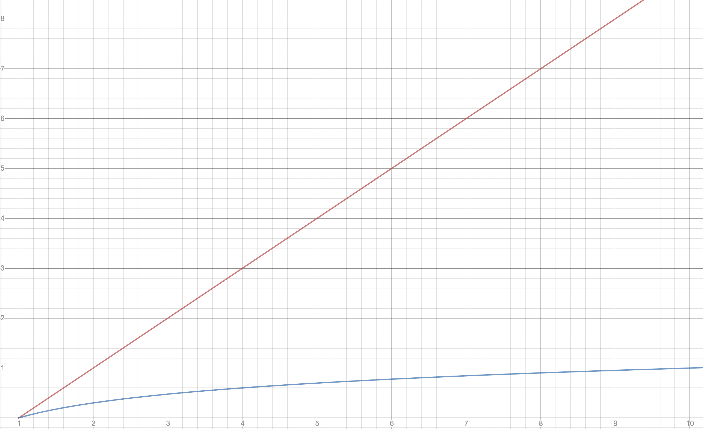
Pictorially, we can see this \(\mathcal{O}(\log(n))\) algorithm runs MUCH faster than an \(\mathcal{O}(n)\) algorithm in the following graph. The x-axis represents \(n\) as it increases and the y-axis shows the approximate number of steps. The red line that grows linearly demonstrates an \(\mathcal{O}(n)\) algorithm while the blue line that shows a slower growth is an example of a \(\mathcal{O}(\log(n))\) function.

To get a sense of just how little \(\mathcal{O}(\log(n))\) grows, consider making a list of values for all 332 million people in the U.S. The run-time for a binary search on this entire list would be approximately 28 steps ! Maybe you might not think the U.S. is THAT big, but a binary search over all 1.4 billion people in China would only take about 30 steps . This is incredibly efficient as \(n\) grows!

Binary Search Trees

While binary search has these really nice scaling properties in theory, there are sometimes some slight modifications we make to the algorithm to work faster in practice when working with large datasets. This section is mostly is inspired by the world of databases, where we usually are managing large amounts of data that might not fit into memory so it will need to be stored on disk (you may have heard of this thing called SQL which is a common language for querying a database).

Note

Here’s a brief recap of memory from Lesson 18: Your computer has memory (sometimes called RAM) which provides relatively fast access to the working data your program leaves. Modern computers have between 4GB and 16GB of RAM. This is opposed to the long-term storage of disk (sometimes called a hard drive or a SSD) which provides much more capacity (>128 GB) but is very slow to access. A big slowdown in data-intensive applications is reading large data files from disk that might not completely fit into your RAM.

Binary search can sometimes be inefficient in practice since it avoids the principle of locality! It jumps around the list and rarely accesses adjacent elements! This means if data has to be constantly read from disk, even though it is asymptotically more efficient, it can be much slower in practice since it can require many disk reads!

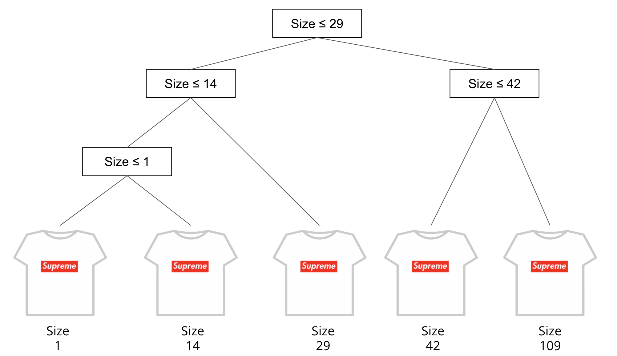
One trick database people have come up with is to make a data structure called a binary search tree that encodes this search information that gets computed once and reused many times. A binary search tree is much like a decision tree from ML, where at each node in the tree you go left/right based on some condition. So for example, in our shirts example, we could construct a tree that records the choices you make during any possible binary search as in the picture below.

This doesn’t involve anything complicated like machine learning to find this tree, it just requires a bit of pre-computing to find the sequence of mid-points for any search. While this does require a bit of work to compute, the idea is that if we compute this tree ahead of time, it can speed up queries later on because they can efficiently traverse down this structure while minimizing the number of times they go to disk to actually look at values in the data.

While it does take a bit of pre-processing to build up the right tree, the binary search tree enjoys the same complexity as binary search. That means if there are \(n\) items to search over, a correctly constructed binary search tree will have a search time of \(\mathcal{O}(\log(n))\) since it will be created by this halving-algorithm.

One of the nice things about this tree structure is it allows you to easily answer range queries. Say if you’re looking for all the shirts between sizes 1 and 42, you can follow the low-end and high-end paths down the tree to find everything in between!

It is probably not super clear why representing this tree concretely as a data structure helps us here, but the databases people have done a TON of work to make this structure efficient for queries. Now that we have some intuition for how a tree-guided search can work, it will be much easier to understand a more complex example that really does require the use of a tree.