Big-O
Contents
Big-O#
Now that we feel a little bit more comfortable counting steps, we can go back to trying to compare sum1 and sum2 . Recall these functions were defined as:
def sum1(n):
    total = 0
    for i in range(n + 1):
        total += i
    return total


def sum2(n):
    return n * (n + 1) // 2
To answer the question of how many steps it takes to run these functions, we now need to talk about the number of steps in terms of the input n (since the number of steps might depend on n ).
Below, we annotate the code with step counting.
def sum1(n):                 # Total: n + 3 steps
    total = 0                # 1 step
    for i in range(n + 1):   # Runs n + 1 times, for a total of n + 1
        total += i           #   1 step
    return total             # 1 step


def sum2(n):                 # Total: 1 step
    return n * (n + 1) // 2  # 1 step
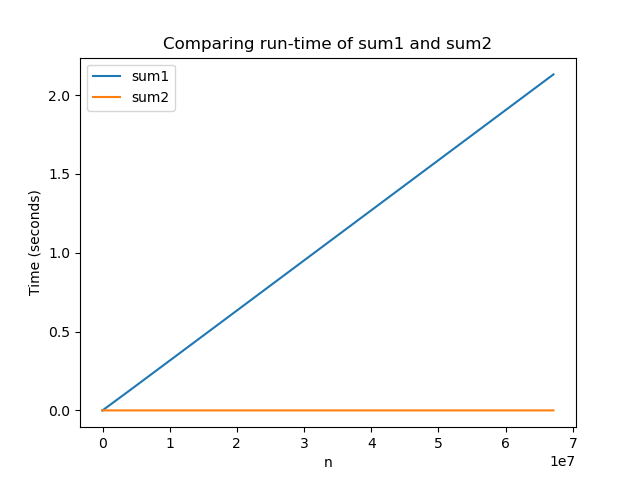
So with this counting rule, sum1(n) runs in n+3 steps while sum2(n) always runs in 1 step!
Amazingly, this weird counting rule matches the graph that we produced earlier with timing code! We saw that sum1 grew proportionally to its input n while sum2 always seemed about the same. With these counting rules, it’s easier to come to that conclusion without having to go through the process of actually timing the code!
Reporting Steps#
Since everything we’ve done with counting steps is a super loose approximation, we don’t really want to promise that the relationship for the run time is something exactly like n + 3 . Instead, we want to report that there is some dependence on n for the run-time so that we get the idea of how the function scales, without spending too much time quibbling over whether it’s truly n + 3 or n + 2 .
Instead, computer scientists generally drop any constants or low-order terms from the expression n + 3 and just report that it “grows like n .” The notation we use is called Big-O notation. Instead of reporting n + 3 as the growth of steps, we instead report \(\mathcal{O}(n)\). This means that the growth is proportional to n but we aren’t saying the exact number of steps.
You get used to this process of dropping information with practice.
Example#
Suppose we did the step counting procedure for some block of code that depends on its input n and counted \(2n^2 + 5n+ 3\) (we can get \(n^2\) from nested loops that both go to n ). Instead of reporting this entire formula, we will report the part that has the biggest impact on its run-time. Out of all the terms, when n is very large, the term \(2n^2\) contributes the most to the overall run-time. This is why we will report \(\mathcal{O}(n^2)\) instead of the whole formula we counted (we also drop coefficients since they don’t matter as much when n is very large).
Another Example#
Consider the folllwing snippet.
def method(n):
    result = 0
    print('Starting method')
    for i in range(9):
        for j in range(n):
            result += i * j
            print(result)
    return result
What is the run-time of this function in Big-O notation? Students will commonly come up with an answer like \(\mathcal{O}(2n^2 + 3)\) which is not correct on two counts:
The first is a common misconception where people assume nested loops mean something like \(\mathcal{O}(n^2)\). This is not the case! This is only true if both loops run \(n\) times! In this case, the outer loop runs 9 times and the inner-loop runs \(n\) times so it will be something on the order of \(9n\) steps, not \(n^2\) steps!
The second is that when you report a Big-O result, you should always drop coefficients in front of terms, and lower-order terms. This formula for steps is wrong in the first place, but assuming it was correct, you would report \(\mathcal{O}(n^2)\) after dropping the coefficient and lower-order terms.
Putting these together, this means the correct answer would be \(\mathcal{O}(n)\)!
Why is this useful?#
Even though it feels weird to throw away things like coefficients and low-order terms, the Big-O notation is helpful because it lets us communicate how our algorithms scale very simply. By scale, we mean quantifying approximately how much longer a program will run if you were to increase its input size. For example, if I told you an algorithm was \(\mathcal{O}(n^2)\), you would know that if I were to double the input size \(n\), that the program would take about 4x as long to run (because of the squared)!
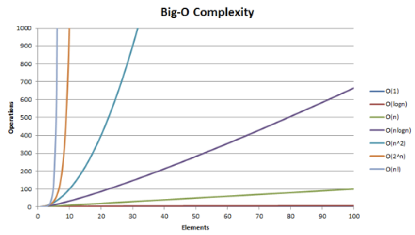
Computer scientists use Big-O notation so much, we consider algorithms by which complexity class they are in. The word complexity is a CS term for Big-O run-time. Here are some common complexity classes
Constant: \(\mathcal{O}(1)\)
If \(n\) doubles, run-time stays the same
Logarithmic: \(\mathcal{O}(\log(n))\)
Grows very slowly
Linear: \(\mathcal{O}(n)\)
If \(n\) doubles, run-time doubles
Quadratic: \(\mathcal{O}(n^2)\)
If \(n\) doubles, run-time quadruples
Cubic: \(\mathcal{O}(n^3)\)
If \(n\) doubles, run-time multiplies by 8
Exponential: \(\mathcal{O}(2^n)\)
Not good… Even for some moderately sized \(n\), say around 200, \(2^n\) is larger than the number of atoms in the observable universe!
It sometimes helps to compare how these things grow pictorially. Below is a graph showing the approximate number of steps for each complexity class as \(n\) increases. Notice which ones grow slowly and which ones shoot off the graph for even small \(n \approx 10\).