Images

---

Data

You can download the dataset used in this reading here:

• duck.jpg

One of the applications of numpy we discussed earlier was representing image data. We will discuss analyzing images and manipulating them for the rest of the module. While we will show some code, the more important bit for this lesson is just the conceptual understanding of how we will represent an image in Python.

Grayscale Images

To start, let’s consider black-white images, which are commonly called grayscale images. Here is a picture of a grayscale dog.

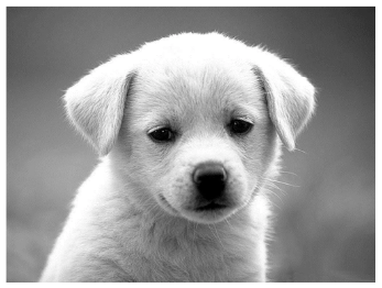
From the computer’s perspective, we think of images as just a big grid of values called pixels . This mirrors how your screen actually displays images! It is a bunch of these pixels that can show a color based on a specified value. For a grayscale image, each pixel needs to know how white or how black it should display.

Conventionally, we represent each pixel as a number between 0 and 255. 0 is the darkest value possible (black) while 255 is the lightest value possible (white). This means a grayscale image is really just a big 2D array of numbers between 0 and 255!

You could imagine a low-resolution image (one with very few pixels) would look something like this

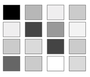
In numpy , we would represent this with a 2D array with values that look something like the following.

[[0, 100, 175, 120],
 [180, 61, 83, 130],
 [118, 137, 59, 121],
 [73, 133, 237, 140]]

Where the values are low, we get darker colors, while where the values are high, we get lighter ones. The dog image above is just a really large 2D array of these values 0 to 255!

Note

At first glance, 255 might seem like an arbitrary number. So where does it come from? It turns out that 255 is the biggest integer that can be stored in a single byte of information. For grayscale images, we typically use one byte to store each pixel in the image. That means saving a grayscale image with ~1000 pixels would take up ~1 kilobyte (i.e. ~1000 bytes) of memory on your computer.

Grayscale Image Code

We are going to use a library called imageio to help read in an image to a numpy array. The following snippet reads in an image, prints some values about it, and then uses a slightly new matplotlib feature to plot an image from a numpy array. We have to pass in a colormap cmap to tell matplotlib to plot the values as grayscale since by default, it uses that yellow/purple color scheme (if you take out the parameter, you can see what it does when you run it!).

The last example in the snippet modifies the array (using slice syntax). Before you open pic2.png , what do you think the image will look like?

import imageio
import matplotlib.pyplot as plt
import numpy as np

# Read in the image
penguin = imageio.imread('/course/lecture-readings/penguin.jpg')

# Print some values
print('Shape', penguin.shape)
print('Top-left pixel', penguin[0, 0])

# Plot image and save it to a file (have to specify to plot as grayscale)
plt.imshow(penguin, cmap=plt.cm.gray)
plt.savefig('pic1.png')

# Modify the numpy array and save that
penguin[350:400, :] = 100

# Plot image and save it to a file (have to specify to plot as grayscale)
plt.imshow(penguin, cmap=plt.cm.gray)
plt.savefig('pic2.png')

Color Images

Let’s brighten up the world a bit and switch to color images. A color image is commonly represented in a format called RGB. RGB stands for “Red, Blue, Green”. An RGB image is really just 3 “grayscale” images stacked on top of each other, but each sub-image corresponds to a particular color channel.

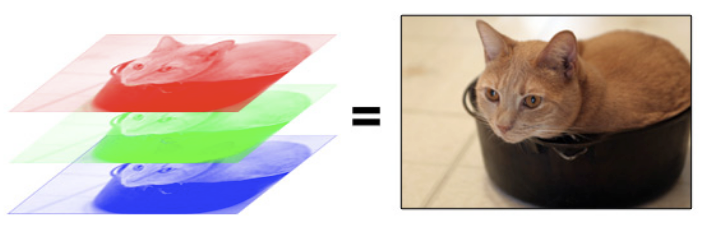
So each pixel in an image is really 3 numbers to tell it how much red, blue, and green respectively to output. Your brain does all the real work of combining how much red/blue/green corresponds to a more complex color like the orange/brown color that the cat is.

In turn, a numpy array will just have to represent all 3 colors for each pixel. Each pixel will store 3 values between 0 and 255; a low value means that color channel is more off (black) while a high value means that color channel is more on (red, blue, or green respectively). Since each pixel needs to know 3 numbers, we will represent this as a 3D numpy.array!

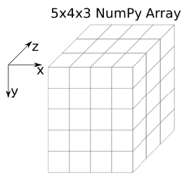
Notice, none of our discussion about numpy actually limits it to 1D or 2D arrays. We can actually have arbitrarily many dimensions! A color image in numpy will commonly be represented as a 3D array with shape (height, width, 3) . The last dimension has shape 3 because there will be one dimension for each color channel at that pixel location. Visually this makes it kind of like a cube that has “depth” 3 (in the z direction).

To index into a color image, you now need to specify 3 values. For example, img[row, col, channel].

Color Image Code

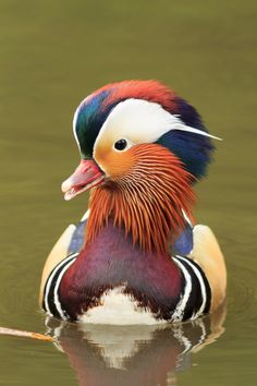
We start with a simple example as we did with grayscale. Notice in this example, the shape printed has 3 dimensions and the third one has shape 3 (for the 3 color channels). As a note, we do not need to specify a cmap since matplotlib does the right thing for 3D numpy.array s by default.

import imageio
import matplotlib.pyplot as plt
import numpy as np

# Read in the image
duck = imageio.imread('duck.jpg')

# Print some values
print('Shape', duck.shape)
print('Top-left pixel: Red =', duck[0, 0, 0])
print('Top-left pixel: Gren =', duck[0, 0, 1])
print('Top-left pixel: Blue =', duck[0, 0, 2])

# Plot image and save it to a file
plt.imshow(duck)
plt.savefig('pic1.png')

Now let’s do something slightly more complex where we modify the colors in the image. Notice in the last example we had to specify three values to index into the image. The same applies here. As we modify each section, we are setting one of the R, G, or B values respectively.

import imageio
import matplotlib.pyplot as plt
import numpy as np

# Read in the image
duck = imageio.imread('duck.jpg')

# Remove red from a row of pixels
duck[100:150, :, 0] = 0

# Remove green from a row of pixels
duck[200:250, :, 1] = 0

# Make a white column by setting all color channels to 0
duck[:, 175:200, :] = 255

# Plot image and save it to a file
plt.imshow(duck)
plt.savefig('pic1.png')