Introduction to Geospatial Data

Data

You can download the dataset used in this reading here:

• geo_data.zip

---

A lot of data we work with is associated with someone or someplace in the real world. Geospatial data is data that contains information about a place in the world.

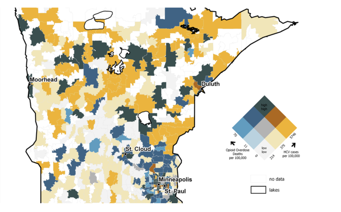
Below is an example plot that shows information about opioid overdoses on top of a map of Minnesota. We don’t have access to the data itself, but we can see something special in this plot: each data point is associated with an area on the map that is shaded depending on its data values. Geospatial information records the areas and shapes of an object to facilitate analysis and visualization.

Introduction to geopandas

A very common format for geospatial data is just a plain CSV that we could parse with pandas . However, they usually also contain a special column to indicate the location in the world that row corresponds to. A very simple representation uses latitude and longitude for each row, but geospatial data can store a very rich set of geospatial features in general.

In order to process this special column format to encode geospatial information, we have to use a new library called geopandas . Don’t worry, everything you know from pandas carries over here with some added on features!

In the code cell below, we show how to load in one of these geospatial datasets with geopandas . The dataset contains information about various countries of the world and information like their population and GDP. The file we will use is a shapefile ( .shp ). The file format itself is actually pretty complex so we will only look at the data after parsing it in geopandas rather than looking at the file directly.

import geopandas as gpd

df = gpd.read_file('geo_data/ne_110m_admin_0_countries.shp')

# Print out the columns
print('===== Columns ======')
print(df.columns)
print()

# Print out one row of data
print('===== First row =====')
print(df.loc[0])

The type of the value df in the cell above is a GeoDataFrame . It behaves exactly like a DataFrame but knows how to do some extra geospatial processing. There is also a GeoSeries type unsurprisingly. To start seeing the power of geopandas , you can see what happens if you ask the GeoDataFrame to plot itself.

import geopandas as gpd
import matplotlib.pyplot as plt

df = gpd.read_file('geo_data/ne_110m_admin_0_countries.shp')

df.plot()
plt.savefig('world.png')

You can get fancier and have it color each country by its population using the column parameter, like in the snippet below.

import geopandas as gpd
import matplotlib.pyplot as plt

df = gpd.read_file('geo_data/ne_110m_admin_0_countries.shp')

# POP_EST is the name of the colummn containing population information
# legend=True makes the legend appear
df.plot(column='POP_EST', legend=True)
plt.savefig('world_population.png')

Geometry

Each row in the data corresponds to one country. The dataset has a special column called 'geometry' that stores the shape of each country with a geometry .

import geopandas as gpd
import matplotlib.pyplot as plt

df = gpd.read_file('geo_data/ne_110m_admin_0_countries.shp')

print(df['geometry'])

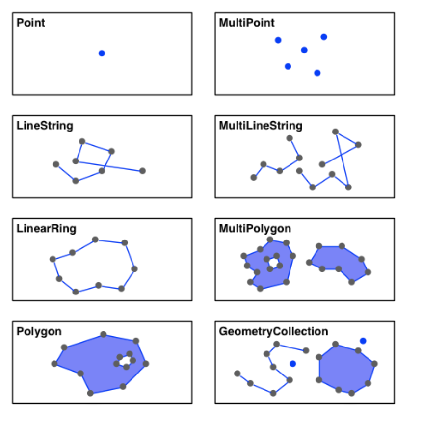
You don’t need to memorize the different types of geometries, but it helps to be familiar with what can be represented in this column. The picture below shows different types of geometries. Most countries are represented by a Polygon or a MultiPolygon (e.g. if they have multiple bodies of land) while you would likely not find any LineString countries in this dataset.