Machine Learning Code

Jupyter Info

Reminder, that on this site the Jupyter Notebooks are read-only and you can’t interact with them. Click the button above to launch an interactive version of this notebook.

• With Binder, you get a temporary Jupyter Notebook website that opens with this notebook. Any code you write will be lost when you close the tab. Make sure to download the notebook so you can save it for later!

• With Colab, it will open Google Colaboratory. You can save the notebook there to your Google Drive. If you don’t save to your Drive, any code you write will be lost when you close the tab. You can find the data files for this notebook below:

  • homes.csv

You will need to run all the cells of the notebook to see the output. You can do this with hitting Shift-Enter on each cell or clicking the “Run All” button above.

Before we begin, let’s put a word of caution about how to approach learning these libraries:

Trying to memorize all of these function calls and patterns is a ridiculous task. We will throw a lot of new functions at you very quickly and the intent is not for you to be able to memorize them all. The more important thing is to understand how to use them as examples and adapt those examples to the problem you are trying to solve.

The most important thing is to understand the big ideas we highlight about the code we are showing!

This means we won’t always be able to explain every bit of code. The purpose is to give you some examples that you can run for your own projects or homeworks, even if you don’t have the hundreds of pages of documentation memorized (because no one acually does that!).

Machine Learning

So far, everything has been awfully abstract and high level. In this notebook, hopefully we can make things more concrete by tying the terms we introduced in the last slide to specific pieces of code to actually train a model. In the next slide, we will introduce the specifics of what this model is learning and how it learns!

For this notebook, we will use a dataset about homes in either San Francisco or New York[1]. This dataset has a row for each house, and some various attributes of the house like which city it’s in, its elevation, and the year it was built.

[1] This data was provided by R2D3 and has been slightly modified to fit our course. Please see the original source for licensing information.

Now, let’s load in this dataset and train a machine learning model to predict the city from the features!

import pandas as pd

data = pd.read_csv('homes.csv')

data.head()

	beds	bath	price	year_built	sqft	price_per_sqft	elevation	city
0	2.0	1.0	999000	1960	1000	999	10	NY
1	2.0	2.0	2750000	2006	1418	1939	0	NY
2	2.0	2.0	1350000	1900	2150	628	9	NY
3	1.0	1.0	629000	1903	500	1258	9	NY
4	0.0	1.0	439000	1930	500	878	10	NY

To train a machine learning model, we will use the popular library scikit-learn (sklearn). sklearn has functions to train and evaluate machine learning models. You’ll see that like seaborn, you won’t end up writing a ton of code to train a model which makes sklearn very convenient to use!

In the last slide, we introduced two questions we have to ask ourselves when applying an ML task.

1. What is your data? Do you have a good set of labeled data to train on? What are the features? What are the labels?

   • Features: All of the columns that describe the house (all but city).

   • Labels: We want to predict which city a house is in from the features, so city is the column that describes that.

2. What are you trying to model? Is this a regression task or a classification task? What model will you apply for that particular task?

   • This is a classification task since we are predicting SF or NY.

   • We haven’t described possible models yet, so we skip this part of the question for now.

Preparing Data

So then the first step in training an ML model, is preparing the data so the model can use it.

We start by separating the data into its features and its labels. Notice we are able to also use masking for the columns we want in pandas! This is a succinct way to keep all the columns that aren’t the label we want to predict ('city').

features = data.loc[:, data.columns != 'city']
labels = data['city']

We can then look at the features we will use.

features

	beds	bath	price	year_built	sqft	price_per_sqft	elevation
0	2.0	1.0	999000	1960	1000	999	10
1	2.0	2.0	2750000	2006	1418	1939	0
2	2.0	2.0	1350000	1900	2150	628	9
3	1.0	1.0	629000	1903	500	1258	9
4	0.0	1.0	439000	1930	500	878	10
...	...	...	...	...	...	...	...
487	5.0	2.5	1800000	1890	3073	586	76
488	2.0	1.0	695000	1923	1045	665	106
489	3.0	2.0	1650000	1922	1483	1113	106
490	1.0	1.0	649000	1983	850	764	163
491	3.0	2.0	995000	1956	1305	762	216

492 rows × 7 columns

And then also the labels.

labels

0      NY
1      NY
2      NY
3      NY
4      NY
       ..
487    SF
488    SF
489    SF
490    SF
491    SF
Name: city, Length: 492, dtype: object

In the cell below, we import a class from sklearn that represents a type of model called a decision tree. The syntax will look a little different than we have seen before since it uses this feature of Python called classes and objects (our topic of study next week).

We won’t explain quite yet what a decision tree is doing, but just treat it like that green plane that separates the cats/dog images from our intro slide (although it will use a slightly different way of separating our SF/NY houses).

# Import the model
from sklearn.tree import DecisionTreeClassifier

# Create an untrained model
model = DecisionTreeClassifier()

# Train it on our training data
model.fit(features, labels)

DecisionTreeClassifier()

Now that we have trained the model, we can now use it to make predictions about new examples! We use the predict function on this model to make a prediction for some examples. Since there are nearly 500 houses in this dataset, we make the predictions on a few specified rows and compare the prediction with the label from the original dataset.

predictions = model.predict(features.loc[::80])
print('Predictions:', predictions)
actual_labels = labels.loc[::80]
print('Actual     :', actual_labels.values)  # To get it to print out the same way

Predictions: ['NY' 'NY' 'NY' 'SF' 'SF' 'SF' 'SF']
Actual     : ['NY' 'NY' 'NY' 'SF' 'SF' 'SF' 'SF']

That looks pretty good! It looks like it is able to accurately make predictions for those examples (since they match the true labels).

sklearn also provides an function called accuracy_score to evaluate how well a model is doing on some dataset. This only works for classification problems, and it returns the percentage of examples the model predicted correctly! You give it both the true labels and the predicted labels, and it computes this accuracy score for you. Accuracy scores will be any number between:

• 0, meaning your model predicted 0% of the labels correctly

• 1.0, meaning your model correctly predicted all labels

from sklearn.metrics import accuracy_score

predictions = model.predict(features)
accuracy_score(labels, predictions)

1.0

Wow! We are able to get 100% of the examples correct! 🎉 Congrats! I guess we have now fully solved ML!

Unfortunately, it turns out that evaluating a model will be a little trickier than this and that we probably shouldn’t expect that this model will get every example it sees in the future correct. How to better assess the models we learn will be the focus of Lesson 12.

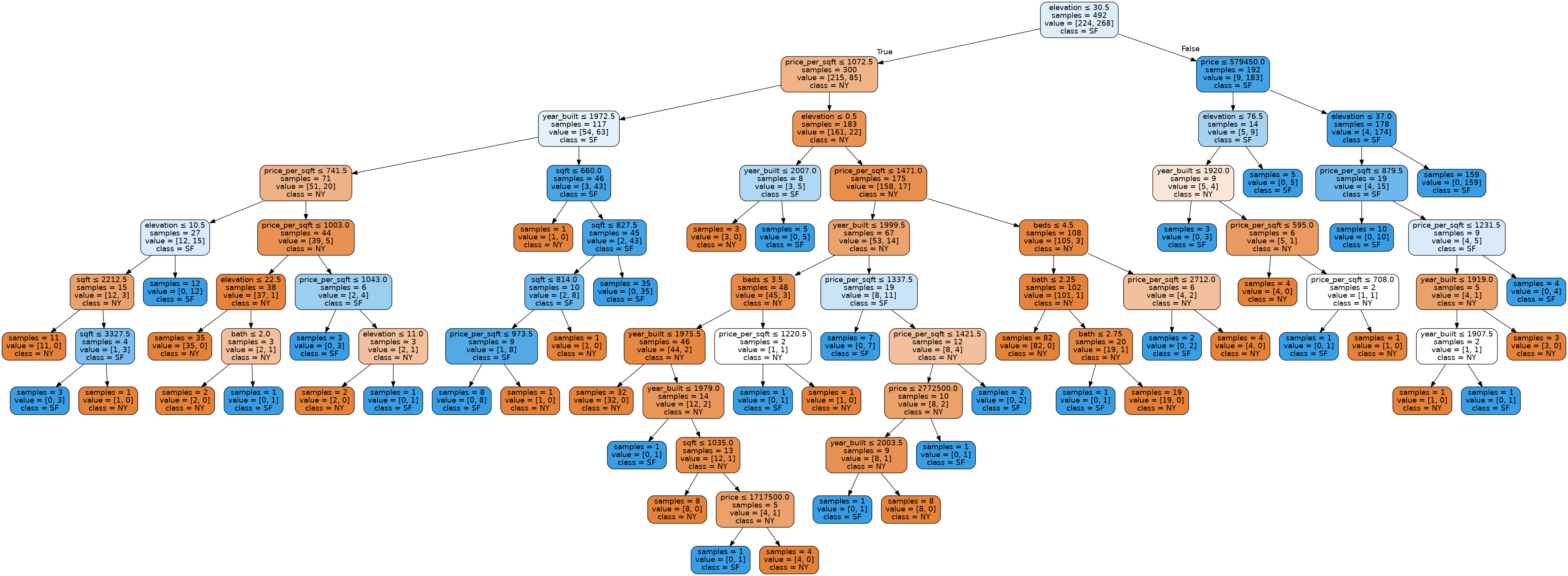
Visualizing The Model

Before we go on to the next slide that explains what this decision tree classifier is, we will quickly show that sklearn provides a way of visualizing what this decision tree looks like! The function plot_tree is not important to understand as it has to use a few advanced library features to get the image to display nicely. You can click on the image to enlarge it.

The next slide talks about how this tree is learned and how you might interpret the output of this image.

from IPython.display import Image, display

import graphviz 
from sklearn.tree import export_graphviz


def plot_tree(model, features, labels):
    dot_data = export_graphviz(model, out_file=None, 
            feature_names=features.columns,  
            class_names=labels.unique(),
            impurity=False,
            filled=True, rounded=True,  
            special_characters=True) 
    graphviz.Source(dot_data).render('tree.gv', format='png')
    display(Image(filename='tree.gv.png'))


plot_tree(model, features, labels)

Recap

We introduced a lot of new concepts and code fragments on this slide. For a quick recap, here are all the “important” bits to train an ML model for this task.

# Impot pandas
import pandas as pd
# Import the model
from sklearn.tree import DecisionTreeClassifier
# Import the function to compute accuracy
from sklearn.metrics import accuracy_score

# Read in data
data = pd.read_csv('homes.csv')

# Separate data into features and labels
features = data.loc[:, data.columns != 'city']
labels = data['city']

# Create an untrained model
model = DecisionTreeClassifier()
# Train it on our training data
model.fit(features, labels)

# Make predictions on the data
predictions = model.predict(features)
# Assess the accuracy of the model
accuracy_score(labels, predictions)

1.0