Spatial Index

---

Now that we have a cursory idea of how to use a tree index to help us find data in a large collection more efficiently, we can now explore how the same principle can be applied to geospatial data.

For this slide, we will focus on just one particular problem in geospatial processing: assume we have a collection of Point s and we want to find if there is a Point in this collection with some given (x, y) coordinates. There are definitely other questions you might be interested in answering efficiently involving geospatial data, but they generally rely on the same principle although their details tend to be more complex. Having a solid understanding of this example with Point s will take you a long way in terms of how to access geospatial data quickly.

For example, assume we had a geospatial dataset that shows the location of Fish & Chips restaurants in the U.K shown in the image below. Each row of the dataset would correspond to one restaurant and would have information like its name, star ratings, and would have a geometry column for the exact Point location of the restaurant. While we could plot this to get a map like the picture shown below, the geometry column is really a GeoSeries of these Point objects, where each Point represents an (x, y) pair of longitude and latitude.

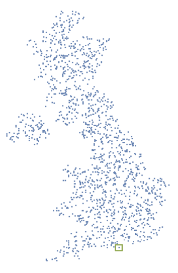
The question we are interested in answering is: Is there a Fish & Chips place at the coordinates (50.809325, -1.368300) ? Now we could pretty easily do this if we just search through the whole geometry column trying to find a Point that matches. However, we are interested in seeing if there is a way to find such a Point without requiring an \(\mathcal{O}(n)\) query.

It turns out we can do a very similar trick as the binary search tree to help us more efficiently find a Point with the given coordinates. This will end up being slightly more complex because there are now 2-dimensions to work with (latitude and longitude), but in spirit, the idea is the same.

Instead of trying to search through every single Point , let’s try to “divide the country in half” to reduce the number of Point s we have to search through. The image below shows an example line that divides the Point s into roughly two equal-sized groups.

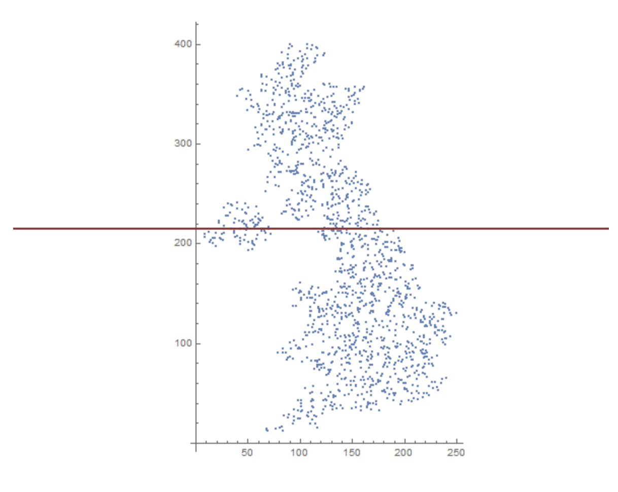
Now, this is helpful, because if we are looking for a particular Point , we just have to ask if it lies above/below that line and we can narrow our search down to half as many points that fall into that group. However, you might be able to tell that this doesn’t help us in terms of the complexity of the search! Searching through \(n/2\) items is still an \(\mathcal{O}(n)\) algorithm!

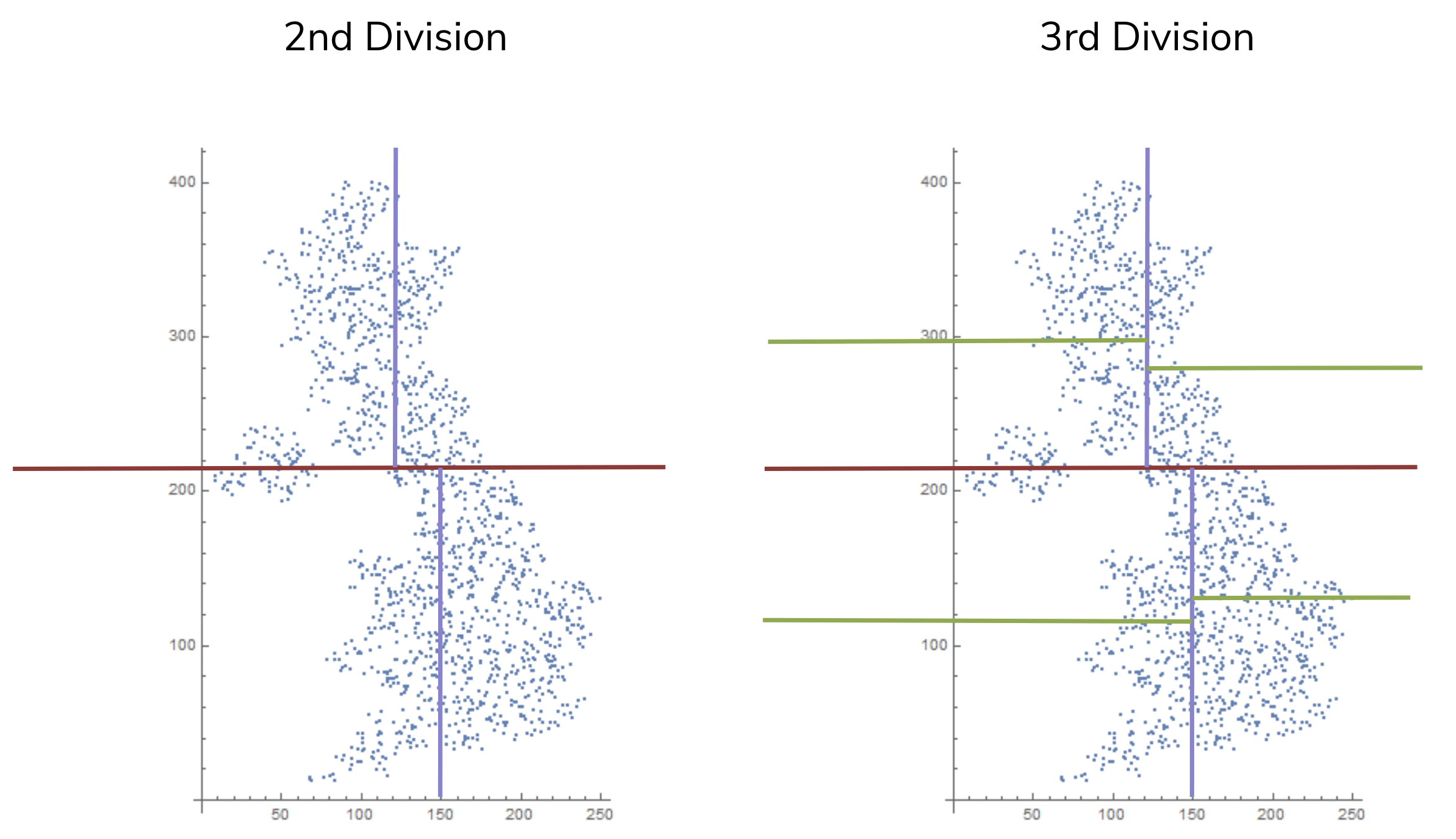
The trick here is to repeatedly divide the groups in half just like we did with the binary search tree! For example, the image below shows what would happen after you split the groups once more and then one more time after that. Technically, you would continue this splitting process, normally switching directions each time, until there was just one Point in each region.

While the idea of splitting the points in half repeatedly might make sense at a very high-level, it’s probably not clear how we would represent these splits so that we could use them later. Trees will come to save the day again! We will represent each of these splits in the data as a split in a tree. This will be very similar to our binary search tree, but the nodes will say something like “latitude < 50” to record which dimension to go up/down/left/right based on.

The picture below shows a smaller example of points that have been divided up and the tree that records these splits. The points are labeled a - g and the splits are labeled with numbers.

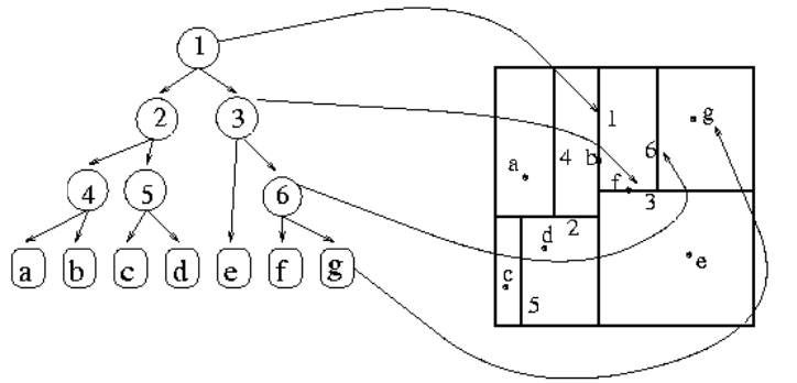
So say we are searching for the point with the same coordinates as g (i.e., we know its (x, y) coordinates, but we do not know which point corresponds to those coordinates).

• We start with the top-level split labeled 1 which corresponds to the vertical line labeled 1 in the image on the right. Since the x-coordinate of our query is to the right of the line 1 , we go to the right in the tree to the node labeled 3 .

• Since the query point is above the horizontal line labeled 3, we follow the tree’s directions and go right to the node labeled 6 . Notice that the tree shown in the picture is not very descriptive since it doesn’t show “above the line 3 ” as “go to the right”, but in practice, this information would be encoded in each node of the tree so it is not ambiguous.

• Since our query point is to the right of line 6 , we go to the right of node 6 in the tree to the node labeled g .

• Since we have reached a leaf node that corresponds to the point g , we can compare our query point to g to see if we found our answer. If their coordinates don’t match, we know our query is not in the dataset.

The name of this 2-dimensional tree is a KD-Tree (for \(k\)-dimensional tree). In essence, this is just an extension of the binary search tree to higher dimensions! The \(k\) in KD-Tree makes it generic so it is a structure that can also help you with 3D or higher-dimensional data.

Efficiency

You might be wondering, is this using a KD-Tree faster than searching through all the points? In general, yes, but there is a pretty big caveat to this. Just like the binary search tree, a KD-Tree will enjoy a query time of \(\mathcal{O}(\log(n))\) since each split will roughly divide the number of points remaining in half. This is nice because if you are going to be querying for points quite frequently, this will result in a faster system.

In general, whenever you add an index on top of your data to make certain queries faster, it comes at a cost (there is no free lunch!). KD-Trees, like most indexes, suffer from the following drawbacks:

• Construction Time: It is non-trivial to build up this tree in the first place. We didn’t describe the algorithm to build up the tree, but it involves sorting the data multiple times in different ways. Without going into the details, to build a KD-Tree with points that are \(k\)-dimensional (where, in our example, \(k\) was 2), requires \(\mathcal{O}(kn\log(n))\) time and \(\mathcal{O}(n)\) space. This is a non-trivial startup cost to build one of these, so it’s only worth it if it will save you time in a system that makes frequent queries.

• Update Time: One of the biggest assumptions we have been making about our search trees is that they are balanced. This means that on both sides of a split, there is the same number of data points (i.e., each split actually splits the data in half). This is relatively doable to achieve if you write a correct algorithm to build the tree but it is much harder to ensure if you are trying to update an existing tree. Say if you have new Fish & Chip restaurants coming in, it is pretty difficult to update the tree to make sure it stays balanced after the update.
  
  It’s a bit harder to quantify the cost of updating an existing tree, but just consider the alternative of updating a simple list of Point s without an index! If a new Point came in and you didn’t have to worry about updating an index to help you find that Point , you could just do something simple like append it to the end. Having an index does speed up search times, but now causes a larger burden for updates. This means people designing data systems need to carefully consider the use case of their system and if an index will help them.

Take Away

Indexing is a very general strategy for letting you query data more efficiently but does come at a startup cost and less flexibility for updates. This is all part of the tradeoffs that come with working with large datasets. In terms of how you actually create these structures, for geopandas they are usually created behind the scenes when you are doing a sjoin . There are some cases where you can explicitly create a geospatial index, but we will not use that for our assignments in this course.

Note

Interested in learning more? There is a great writeup on how to do this with GIS data here . Note that his reading talks about “R-trees” while we talked about “KD-trees”. R-trees are very similar, but are made by making a series of rectangeles (also called bounding boxes), while our KD-trees were made by a series of dividing lines. Very similar in intent, but just slightly different details on execution.