Jittering (Laplace Mechanism)

In the video about the Census, they described the process of jittering published statistics to ensure differential privacy. The act of “jittering” the data is adding some amount of random noise to the published statistics, to add uncertainty in the world about what the true value is. It turns out that there is a very simple procedure for jittering that tells you exactly what level of differential-privacy you can expect from your result.

So let’s take the example of the Census, and publishing some demographic statistic about the US population. So suppose for the sake of example, the true average age of the US population is 38.1 years. If we want to guarantee our published statistic is \(\varepsilon\)-differential private we need to add a little bit of random noise to this value (a.k.a “jittering” the value).

Recall for us to meet \(\varepsilon\)-differential privacy, we need to make sure the result from including a single person vs the result from not including them are similar and \(\varepsilon\) is our control for how similar they have to be; if \(\varepsilon\) is small (near 0), the results must closely match and if it is large, we allow more deviation (e.g., less private).

So much noise do we need to add to make sure our analysis result respects \(\varepsilon\)-differential privacy? It turns out that there is a well defined formula for this using a concept called the Laplace Distribution. You don’t need to understand the details of this distribution but that it’s a random number generator that outputs values; it’s somewhat similar to a normal distribution (or “bell curve”) in that some values near the center or more likely, but the shape of it looks slightly different. If you’re curious, the formula for the distribution for some parameter \(\varepsilon\) is \(f(x) = \frac{\varepsilon}{2}e^{-\epsilon |x|}\). The graph below shows the likelihood of seeing particular values for settings of \(\varepsilon= 0.5, 1, 2\).

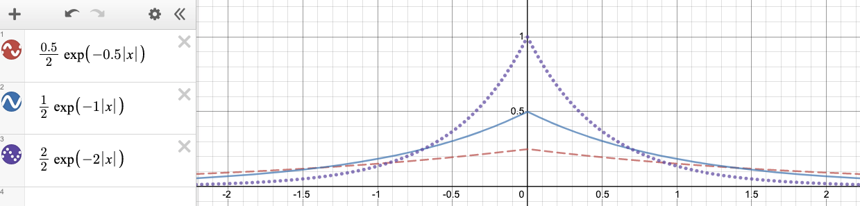
You can see in this graph that the probability of outputting a value near 0 is highest for all three settings of \(\varepsilon\), but the higher \(\varepsilon\) is (e.g., when it’s 2 with the purple dotted lines), it’s much more likely to be near 0 than farther away. While the formula is not important to memorize, this general trend that higher \(\varepsilon\) is this formula makes the random noise closer to 0 is important (we’ll explain why in a second).

It turns out, adding noise that follows this Laplacian distribution is all you need to do! So you take your real statistic, which in our example was 38.1, you add some noise that is a number you generate from the Laplace distribution , and then you report that jittered number instead. So if your random number generator (following a Laplace distribution) output the random value 0.25, you would report 38.35 years as the average age for people.

It turns out this Laplace distribution has a very special property. If you take your statistic you calculated (e.g., average age) and add some noise that came from a Laplace distribution with parameter \(\varepsilon\), your reported statistic satisfied \(\varepsilon\)-differential privacy! We can’t prove that fact so we will have to take it as a given, but we provide some intuition for this below.

To think about the intuition why, think back to what it means for something to be \(\varepsilon\)-differentially private. If \(\varepsilon\) is near 0, then to be \(\varepsilon\)-differentially private, we need there to be very little change in the inclusion/exclusion of someone’s individual data. To meet this, you might expect that the random noise we add needs to be larger to better obsfucate the contribution of a single person to the result of the data. It turns out that for the Laplace distribution, the smaller the parameter \(\varepsilon\) is, the more “spread out” the distribution is. Since it’s less peaked near 0, that means it’s more likely to return a value far away from zero (e.g., more noise). The exact opposite happens for if \(\varepsilon\) is large: we require less similarity with and without someone’s data, and so it is okay if we add noise that is more likely to be near 0.

So to be clear, the important thing here is not to understand the exact formula for the Laplace distribution. The big idea is to understand that you can achieve \(\varepsilon\)-differential privacy on any statistic you publish by adding noise that follows a Laplace distribution with parameter \(\varepsilon\). You should also have an intuitive sense for how which values of noise are more likely than others as you change this parameter \(\varepsilon\) and how that lines up with our definition of differential privacy.