Matplotlib Plotting

---

We have already seen how to make plots using seaborn to make simple data visualizations and using matplotlib to customize the titles and axes. This week, we are going to explore matplotlib a little more in-depth so we can understand how to make even richer visualizations.

Before, when we were using seaborn , whenever we were plotting, we were plotting on a global figure behind the scenes. Some of you might have experienced bugs on HW3 where you used different functions than we instructed. These bugs stem from how different functions interact with this figure. Just like seaborn , pandas has a way to make simple plots that, by default, also plot on a global figure. Take the following toy-example:

import matplotlib.pyplot as plt
import pandas as pd

df = pd.DataFrame({
    'a': [1, 2, 3],
    'b': [1, 2, 3],
    'c': [3, 2, 1]
})

df.plot(x='a', y='b')
df.plot(x='a', y='c')

plt.savefig('plot.png')

This only produced one plot because the second one overwrote the first one on this global figure! If we want to plot these on the same figure, we would need something a little more complex.

A figure is a matplotlib term for a canvas to store the drawings. A figure may have one or more axes and each axis can have multiple plots drawn on it. You can make very interesting visualizations by putting multiple axes on a single figure. Instead of using the default-global figure from seaborn, we have a way to create our own using matplotlib. The code looks like the following.

import matplotlib.pyplot as plt
import pandas as pd

df = pd.DataFrame({
    'a': [1, 2, 3],
    'b': [1, 2, 3],
    'c': [3, 2, 1]
})

# Make a figure with one axis
fig, ax = plt.subplots(1)

# Use the special param `ax` to tell pandas which axis to draw on
df.plot(x='a', y='b', ax=ax)
df.plot(x='a', y='c', ax=ax)

# Ask the figure to save itself
fig.savefig('plot.png')

Notice that the code is mostly the same, but now we explicitly tell pandas to plot on the axis we created. The ax parameter for plot instructs the plotter to use that particular axis to draw on.

Subplots

From what we have seen so far, it’s not very clear why we need to distinguish between a figure and axis. It becomes more clear when you want multiple axes on a single figure. You should think of the figure being the whole window that you can plot in and each axis as being a single set of x/y axes. If you wanted two plots side-by-side, you would have one figure and two axes.

For example, to plot the same graphs as above side-by-side, we could write code like the following.

import matplotlib.pyplot as plt
import pandas as pd

df = pd.DataFrame({
    'a': [1, 2, 3],
    'b': [1, 2, 3],
    'c': [3, 2, 1]
})

# Make a figure with one axis
fig, [ax1, ax2] = plt.subplots(2)

# Use the special param `ax` to tell pandas which axis to draw on
df.plot(x='a', y='b', ax=ax1)
df.plot(x='a', y='c', ax=ax2)

# Ask the figure to save itself
fig.savefig('plot.png')

The subplots call returns a Figure and a list of Axes objects. In this case, we asked for a subplot with 2 Axes objects, so it returned them as a list. We had each call to plot use a different Axes to draw on. The Figure still holds both of the Axes , so to save the figure we will ask the Figure to do that.

subplots is actually really generic in the sense that you can make as many axes as you want! subplots takes two optional parameters nrows and ncols to specify how many rows and columns of axes you want. The returned list of Axes will be a list of lists if you ask for multiple rows and multiple columns.

import matplotlib.pyplot as plt

fig, axs = plt.subplots(nrows=3, ncols=2)
print(axs)

print('Num rows', len(axs))
print('Num cols', len(axs[1]))

If you wanted to visualize this return value, it would look something like this:

[
  [ax1, ax2]
  [ax3, ax4]
  [ax5, ax6]
]

This is an example of a 2d-array (or a list of list s). This is actually using a library we will dive deeper into in the next module, called numpy . This numpy array allows you to access a specific row/column with the bracket notation. For example axs[0, 0] is the top left axes ( ax1 in the output above). In general, the syntax is axs[row, col] where row 0, column 0 is the top left and the rows increase going down and columns increase going right; for example, axs[2, 1] would be ax6 in the output above.

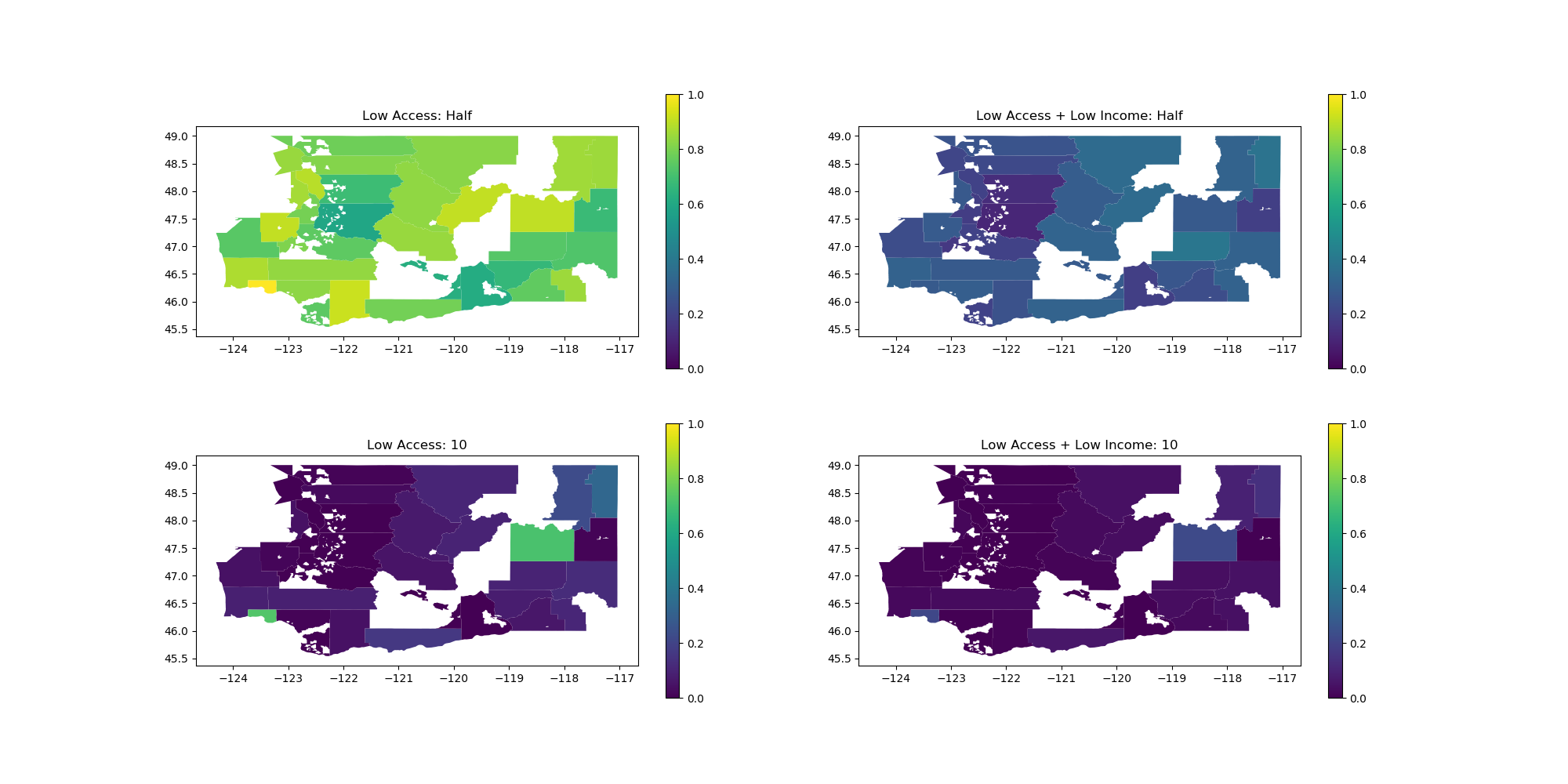
For example, you will be making a plot like the following on your next take-home assignment.

Subplots Examples

There are generally two ways of working with axes return of subplots , index into it or unpack it. For example, the following snippet shows how to make two small plots using both styles.

import matplotlib.pyplot as plt
import pandas as pd

# Make the data
df = pd.DataFrame({
    'a': [1, 2, 3],
    'b': [1, 2, 3],
    'c': [3, 2, 1]
})

# Option 1: Index into the structure
fig, axs = plt.subplots(nrows=2)
df.plot(x='a', y='b', ax=axs[0])
df.plot(x='a', y='c', ax=axs[1])
fig.savefig('option1.png')

# Option 2: Unpack the axes
fig, [ax1, ax2] = plt.subplots(nrows=2)
df.plot(x='a', y='b', ax=ax1)
df.plot(x='a', y='c', ax=ax2)
fig.savefig('option2.png')

Usually either suffices, but if you start getting more than 4 or so plots, the second option becomes unwieldy. Below, we show a similar example but with a 2x2 plot.

Before you run the code snippet below, think about what the final plot should look like; when we plot a and b , it is a line with a positive slope ( / ) and when we plot a and c , it is a line with a negative slope ( \ ).

import matplotlib.pyplot as plt
import pandas as pd

# Make the data
df = pd.DataFrame({
    'a': [1, 2, 3],
    'b': [1, 2, 3],
    'c': [3, 2, 1]
})

# Option 1: Index into the structure
fig, axs = plt.subplots(nrows=2, ncols=2)
df.plot(x='a', y='b', ax=axs[0, 0])  # Top-left
df.plot(x='a', y='c', ax=axs[0, 1])  # Top-right
df.plot(x='a', y='c', ax=axs[1, 0])  # Bottom-left
df.plot(x='a', y='b', ax=axs[1, 1])  # Bottom-right
fig.savefig('option1.png')

# Option 2: Unpack the axes
fig, [[ax1, ax2], [ax3, ax4]] = plt.subplots(nrows=2, ncols=2)
df.plot(x='a', y='b', ax=ax1)  # Top-left
df.plot(x='a', y='c', ax=ax2)  # Top-right
df.plot(x='a', y='c', ax=ax3)  # Bottom-left
df.plot(x='a', y='b', ax=ax4)  # Bottom-right
fig.savefig('option2.png')